by Mark Grundland
Email: Mark@Eyemaginary.com
Project for Computational
Geometry CS308-507A
School of Computer Science
at McGill University
Version 1.00
November 1997
| Introduction | ||
| Voronoi Diagrams | ||
| Step 1: Initialization | ||
| Step 2: Tiling | ||
| Step 3: Rendering | ||
| Future Development | ||
| Bibliography |
| |
|
|
Before |
During |
After |
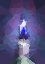
This technical document is meant as a tutorial explaining how VoronoImage creates its stained glass panels. Before reading about how the program works, you should be familiar with what it is trying to do (see the on-line "VoronoImage Operating Manual"; for examples of artwork produced with VoronoImage visit the on-line "VoronoImage Picture Gallery").
The central task of VoronoImage is designing a mosaic of colored tiles and then successively rendering each level of image detail. The colors of the tiles and the detail elements they contain blend together to form the finished stained glass panel. Notice that these detail elements bear a similarity to the mosaic tiles, as each is a polygonal tile taking its color characteristics from some site in the input picture. Just as the mosaic tiles form a partition of the enclosing picture frame, so each polygonal element of the first level of detail is inscribed in one of the mosaic tiles, and likewise each polygonal element of the second level of detail is contained in some element belonging to the first and so on. Finally each image pixel is but a square contained in one of the polygonal elements of the final level of detail. The picture that emerges is a fractal partition of the image into polygonal tiles, with each polygonal tile of each level being partitioned into the tiles of the next level. This structure is essentially a plane partition tree, where every parent tile is partitioned into its children tiles. Each level of the tree corresponds to the polygonal tiles of that level of detail. So the picture frame is the root, the mosaic tiles are its children, and the image pixels are attached to the leaves.
The uniform structure of the tree allows for an effective general strategy for creating the stained glass panel. Begin by generating a set of lists of potential partition tree nodes, first the mosaic tiles and then the lists for each of the subsequent levels of detail. Every node stores the color characteristics of the corresponding site in the input picture. Next build up the tree, one level at a time, by resolving the boundaries between the polygonal tiles. Finally, color each pixel by appropriately blending the colors of its ancestor tiles in the partition tree.
For the purpose of creating a stained glass panel, a suitable partition of the plane into polygonal tiles should have the following desirable properties:
VoronoImage owes its name to Voronoi diagrams, a simple but versatile kind of space partition which satisfies the above requirements. VoronoImage represents a convergence of two techniques. Among the standard plug-ins for the popular image processing program Adobe PhotoShop, the Crystallize plug-in partitions an image into crystalline facets, each a convex polygon colored with the dominant color of the image segment it covers. By rendering details within the mosaic tiles and allowing greater control over the entire effect, VoronoImage is both more powerful and flexible. The second idea is due to the work of Ken Sheriff, who suggests recursively nesting Voronoi diagrams inside Voronoi polygons to create intricate patterns resembling leaf veins or cracked pottery glaze. Whereas he varies the line thickness of the polygons, VoronoImage uses color blending to capture the fractal nature of the structure.
Voronoi diagrams have been studied from as early as 1644 by Descartes. They are now a basic geometric tool which finds applications in many areas of science, from biology to robotics, from physics to geography. Given a list of sites in the plane, a Voronoi diagram assigns each point in the plane to its nearest site. The result is a subdivision of the plane. The Voronoi polygon around each site consists of the points closer to that site than to any other site. As usual, the measure of distance is Euclidean. Unlike some of the other distance metrics, the Euclidean metric promotes a certain visual consistency between the layout of the sites and the resulting convex Voronoi polygons (for example, with the Manhattan distance metric, the Voronoi polygons are no longer guaranteed to be convex). Here's an example of a set of sites and their Voronoi diagram:
Voronoi diagrams are typically calculated by examining the arrangement of bisecting lines formed between each pair of sites. As every bisector divides the plane into two regions, one half-plane composed of points closer to one site and the other half-plane composed of points closer to the other site, so each Voronoi polygon can be viewed as an intersection of all the half-planes of its site. As usually only a few of the many possible half-planes need to be examined to determine the boundaries of the Voronoi polygons, so the optimal algorithms, like the sweep line algorithm and the divide-and-conquer algorithm, both have a worst case running time of O(n log n) in the number of sites. However, in practice, the known optimal algorithms, suffering from the overhead of complex data structures, aren't particularly easy to implement. For the purposes of VoronoImage as well as many other applications, it is sufficient to calculate a discreet Voronoi diagram. Here we are concerned with discreet pixels in a uniform square grid rather than points lying in a continuous plane. The boundaries between Voronoi polygons need only to be known approximately down to the size of a pixel. VoronoImage uses a simple distance mapping algorithm, adapted from a paper by Per-Erik Danielsson, for calculating the discreet Voronoi diagrams. Unlike some of the other approximation approaches based on cellular automata, by actually calculating the Euclidean distances between pixels, this algorithm avoids any cumulative errors. Though rare local errors are possible, they are unobtrusive, never extending beyond isolated pixels. The algorithm is also very fast, with its running time directly proportional to the size of the image and virtually independent of the number of sites.
For more information about what's possible with Voronoi diagrams visit the Geometry Junkyard.

The VoronoImagination application, which performs all of the calculation, starts off by examining the configuration information that the user entered through the VoronoImage stack. The input picture file is read into an offscreen bitmap for color sampling. Next, for the mosaic tiles and each of the subsequent levels of detail, lists of sites are generated. Each site will correspond to a polygonal tile, a location in the image as well as a node in the plane partition tree. Hence each tile record stores the x and y coordinates of the tile's site, the color of the pixel in the input image at that location, the level at which the tile node will be found in the partition tree, and the pointer to the parent tile. With the origin at the center of the image, polar coordinates are used to generate the random tile site locations, allowing for better control over their spatial distribution (this approach is used to implement the focus of detail feature). The pixels are simply pointers to tiles. Initially they all point to a single tile representing the picture frame.

This method of creating a Voronoi diagram is based on a simple intuitive picture. Imagine the still surface of a pond on a windless day. Let raindrops fall from the sky, striking the water simultaneously at a number of sites. Circular ripples emanate from each of the sites. Points on each wave's edge are equidistant to its source. With each wave spreading outwards at the same rate, wherever the waves don't collide, the ripple diameters are equal for all sites at each moment in time. Where two waves meet there will be an edge of the Voronoi diagram. Where more than two waves meet there will be a vertex of the diagram. Each Voronoi polygon can be thought as the ideal maximal extent of the ripple originating from its site. Notice that this scheme is well suited for parallel computation. The essential idea is to let each Voronoi polygon progressively extend outwards from its site. The implementation relies on successively scanning pixels and carefully keeping track of the growing partition tree. Here is the detailed algorithm, along with an example showing the intermediate steps of creating the mosaic tiles within a black picture frame tile:
CreateTiling(pixel array image)
This procedure, invoked for each level of detail, positions the tiles of the corresponding level of the partition tree and determines the resulting subdivision of the image. It calculates the discreet fractal Voronoi diagram for the image array of pixels, where each pixel image[x,y] is attached to its tile image[x,y].tile in partition tree. Note that the x-axis goes from left to right, while the y-axis goes from top to bottom.for each tile t to be placed at the current level of the partition tree
if image[t.x,t.y].tile.level != current level then
Tile Placement Loop: The tiles that will comprise the current level of the partition tree now become the new leaves of the tree, with their sites planted in the image as "seeds" so that the tiles may subsequently grow outwards, from single pixel sites to a polygonal subdivision. The current state of the image reflects a partition of pixels among the tiles of the previous level of the partition tree. Each new tile t finds its parent tile, the tile inscribing t, by examining the current state of the pixel corresponding to the new tile's site. Henceforth that pixel image[t.x,t.y], located at the site's position t.x,t.y, will belong to the new tile t. We must guard against the possibility of two randomly generated sites falling on the same pixel, both belonging to tiles at the same level of the partition tree. Also there may be certain irregularities in the partition tree. It is possible that some tiles of the previous level of the partition tree will contain none of the sites of the tiles of the new level, and hence they won't be subdivided into any of the new tiles; in effect, some branches of the partition tree will appear to skip over some levels of detail. The algorithm takes proper account of these concerns.
for y:= 2 to ymax
Downward Scan Loop: From their single pixel sites, each of the new tiles, comprising the latest level of the partition tree, now expands downwards and outwards to the nearest adjacent pixels, while respecting the boundaries of its inscribing parent tile as well as the other leaf tiles. Of all the tiles which have so far managed to reach a given pixel, the pixel is assigned to the one with the closest site. The algorithm proceeds downwards along a scan line: the first loop compares each scan line pixel with one above it, the second loop successively compares each scan line pixel with the one to the left, and the third loop in the reverse order compares each scan line pixel with the one to the right.
for y:= ymax-1 down to 1
Upward Scan Loop: Likewise, each of the new tiles, comprising the latest level of the partition tree, now expands upwards and outwards to the nearest adjacent pixels, while respecting the boundaries of its inscribing parent tile as well as the other leaf tiles. Some of the tile boundaries will be revised accordingly. The algorithm proceeds upwards along a scan line: the first loop compares each scan line pixel with one below it, the second loop successively compares each scan line pixel with the one to the left, and the third loop in the reverse order compares each scan line pixel with the one to the right.
CompareTiles(target pixel p, target tile t, alternative tile a)
This procedure decides whether to assign pixel p, currently belonging to tile t, to another tile a.if a.level < current level then exit
The pixels should be attached to the leaf tiles of the current partition tree, hence if the alternative tile a is not a leaf tile then it is ignored.else if (t.level < current level) and (t == a.parent) then
Each time the partition tree grows by a new level of tiles, the pixels remain attached to their parent tiles. Suppose this is the case and pixel p is currently attached to the parent tile t of the new leaf tile a. Since this relationship ensures that the leaf tile a is inscribed in the pixel's current tile t, so it is safe to attach tile a to pixel p.else if (t.parent == a.parent) and (distance(p, t.site) > distance(p, a.site)) then
In a discreet Voronoi diagram, the polygonal tile with its site closest to pixel p is the one which must contain the pixel. So if tiles t and a are both leaf tiles having the same inscribing parent tile in the partition tree, the pixel p is assigned to whichever tile has its site closest to p.
The correctness of this approach relies on the fact that a tile as well as its inscribing polygon are both convex and hence monotonic in all directions. By use of the scan line, the algorithm guarantees that while each tile is being constructed it always remains monotonic in both the vertical and the horizontal directions. Within every convex Voronoi polygon, each point may be reached from the polygon's site by a "Manhattan path", proceeding first vertically then horizontally. Through the successive vertical movement of the scan line and the consecutive sequence of horizontal comparisons along it, the algorithm ensures that every expanding tile will spread from its initial site along the correct Manhattan path to reach each of its pixels. Once a pixel is assigned to its correct tile, no other tile may claim it.
The limits of this approach are the limits of using discreet pixels. Regions of the Voronoi polygons that are narrower than the width of a pixel simply can't be seen. Also it is possible that some isolated pixels are assigned to the wrong tiles. In the paper by Per-Erik Danielsson, it is estimated that the error, the difference between the distance from the pixel to the site of its assigned tile and to the site of its correct tile, will never exceed 0.58578 pixel units. These pixels will be found at the sharp vertices of tiles. A pixel may only belong to a tile if at least one of its cardinal neighbors (upper, lower, left, and right pixels) also belongs to the same tile, allowing the Manhattan path from the tile's site to the pixel to pass through its neighbor. But at a tile vertex, all four cardinal neighbors may rightly belong to different tiles. Then the center pixel may or may not be assigned to its correct tile, depending on the exact order in which the tiles spread out. If such a bad center pixel is assigned to its correct tile (see example below), the problem only gets worse. When the partition tree grows to the next level, a new set of tiles will need to be spread out within the confines of this parent tile. None of these new tiles will be able to reach the bad pixel since each of the pixel's cardinal neighbors now belongs to a different parent tile. Also it is possible that the only site of a new tile of the next level to fall on the bad pixel's tile, will choose to fall on the bad pixel. Such a new tile would be unable to spread out, leaving behind a parent tile which is not entirely covered by its children.
Fortunately, testing shows that all these potential irregularities of the partition tree are rare. Even when they do occur, the implemented algorithms are robust enough to ensure that they never visibly affect the outcome. Since their causes are predictable and easy to isolate, other applications using the same algorithms could eliminate them altogether.
Each pixel in the stained glass panel needs to be colored by appropriately blending the colors of all the tiles which contain it. Hence the input picture will be rendered into the angular forms of stained glass, as each tile derives its color from its site's color in the input picture. For every level of the partition tree, from the mosaic tiles down to the subsequent levels of detail, there is at most one tile which contains a given pixel. These tiles comprise the pixel's branch of the partition tree. With the state of the image pixels reflecting the last level of the subdivision, the pixel is attached to the leaf tile of its branch. The other ancestor tiles are simply found by traversing the chain of parent pointers up the pixel's tree branch. Notice that once we have determined the color of one pixel of a leaf tile, we can store this value and use it for the other pixels contained in this tile.
The problem is to arrive at a weighted blend of the tile colors. To maintain the dominance of a mosaic of stained glass tiles over the many other tiles representing the various levels of detail, the mosaic tiles must be given a greater influence in deciding pixel colors than those other tiles. The distribution of weights among the levels of the partition tree affects the overall appearance of the stained glass panel (this is used to simulate the effect of the user's choice of the glass type). The color blending function must ensure that the weights have a predictable and visually meaningful effect as well as that the generated colors are consistent with those in the input image. After all, if the input image contains only patches of blue and red, so the the stained glass panel may include tiles having different shades of red and blue but no bright purple or pink. Using the usual hardware-oriented RGB color model, where each color is composed of red, blue and green components, experiments with different schemes involving weighted sums and products showed that the resulting color blends were difficult control properly. Instead VoronoImage uses the perceptually based HSV color model, where each color is composed of hue (pigment), saturation (intensity) and value (brightness) components. A blend is controlled by three different sets of weights, each for a different color component. The saturation and value components of the blend are simply calculated via weighted sums. The hue component of a color is a unit direction vector, describing an orientation on a color wheel (red at 0° and 360°, green at 120°, blue at 240°). A hue vector is constructed by giving this direction vector a length proportional to the hue's weight. A vector sum of the hue vectors of the tile colors is then calculated. Its unit direction vector becomes the hue component of the blend. With sensible weights, this scheme virtually eliminates the possibility of visually anomalous colors.

Now that the stained glass panel is rendered in an offscreen bitmap, it must be saved as a PICT image file. This output file should have the same color depth as the input file. But, due to the blending of colors, the stained glass panel may actually use many more colors than the original image. In such cases, color sampling and dithering will be applied. Fortunately, the Macintosh Quickdraw graphics system provides a basic level of support for these functions.
Here are some possibilities for the future development of VoronoImage:
Per-Erik Danielsson. Euclidean Distance Mapping. Computer Graphics and Image Processing, 14:227-248, 1980.
M. de Berg, M. van Kreveld, M. Overmars, O. Schwarzkopf. Computational Geometry: Algorithms and Applications. Springer-Verlag, Berlin, 1997.
Ken Shirriff. Generating fractals from Voronoi diagrams. Computers & Graphics, 17:165-167, 1993.
VoronoImage Package: Copyright © 1997 Mark Grundland. All rights reserved.